Interpreting a linear classifier
Notice that a linear classifier computes the score of a class as a weighted sum of all of its pixel values across all 3 of its color channels. Depending on precisely what values we set for these weights, the function has the capacity to like or dislike (depending on the sign of each weight) certain colors at certain positions in the image. For instance, you can imagine that the “ship” class might be more likely if there is a lot of blue on the sides of an image (which could likely correspond to water). You might expect that the “ship” classifier would then have a lot of positive weights across its blue channel weights (presence of blue increases score of ship), and negative weights in the red/green channels (presence of red/green decreases the score of ship).
Another Interpretation of linear classifiers as template matching
Another interpretation for the weights WW is that each row of WW corresponds to a template (or sometimes also called a prototype) for one of the classes. The score of each class for an image is then obtained by comparing each template with the image using an inner product (or dot product) one by one to find the one that “fits” best. With this terminology, the linear classifier is doing template matching, where the templates are learned. Another way to think of it is that we are still effectively doing Nearest Neighbor, but instead of having thousands of training images we are only using a single image per class (although we will learn it, and it does not necessarily have to be one of the images in the training set), and we use the (negative) inner product as the distance instead of the L1 or L2 distance.
Analysis of linear classification
Additionally, note that the horse template seems to contain a two-headed horse, which is due to both left and right facing horses in the dataset. The linear classifier merges these two modes of horses in the data into a single template. Similarly, the car classifier seems to have merged several modes into a single template which has to identify cars from all sides, and of all colors. In particular, this template ended up being red, which hints that there are more red cars in the CIFAR-10 dataset than of any other color. The linear classifier is too weak to properly account for different-colored cars, but as we will see later neural networks will allow us to perform this task. Looking ahead a bit, a neural network will be able to develop intermediate neurons in its hidden layers that could detect specific car types (e.g. green car facing left, blue car facing front, etc.), and neurons on the next layer could combine these into a more accurate car score through a weighted sum of the individual car detectors.
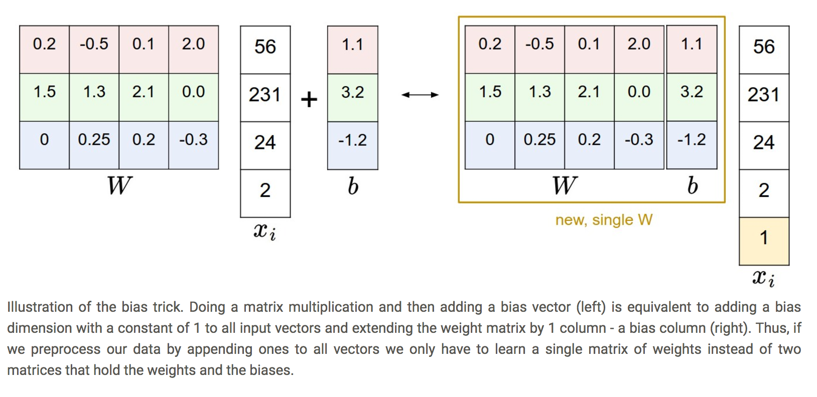
Bias trick
Illustration of the bias trick 
Image data preprocessing
As a quick note, in the examples above we used the raw pixel values (which range from [0…255]). In Machine Learning, it is a very common practice to always perform normalization of your input features (in the case of images, every pixel is thought of as a feature). In particular, it is important to center your data by subtracting the mean from every feature. In the case of images, this corresponds to computing a mean image across the training images and subtracting it from every image to get images where the pixels range from approximately [-127 … 127]. Further common preprocessing is to scale each input feature so that its values range from [-1, 1].
hinge loss, squared hinge loss
- hinge loss: max(0, -)
- squared hinge loss: max(0, -)^2