Note: all the content comes from http://cs231n.github.io/convolutional-networks/
A simple ConvNet is a sequence of layers, and every layer of a ConvNet transforms one volume of activations to another through a differentiable function. We use three main types of layers to build ConvNet architectures: Convolutional Layer, Pooling Layer, and Fully-Connected Layer (exactly as seen in regular Neural Networks). We will stack these layers to form a full ConvNet architecture.
INPUT [32x32x3] will hold the raw pixel values of the image, in this case an image of width 32, height 32, and with three color channels R,G,B.
CONV layer will compute the output of neurons that are connected to local regions in the input, each computing a dot product between their weights and a small region they are connected to in the input volume. This may result in volume such as [32x32x12] if we decided to use 12 filters.
RELU layer will apply an elementwise activation function, such as the max(0,x)max(0,x) thresholding at zero. This leaves the size of the volume unchanged ([32x32x12]).
POOL layer will perform a downsampling operation along the spatial dimensions (width, height), resulting in volume such as [16x16x12].
FC (i.e. fully-connected) layer will compute the class scores, resulting in volume of size [1x1x10], where each of the 10 numbers correspond to a class score, such as among the 10 categories of CIFAR-10. As with ordinary Neural Networks and as the name implies, each neuron in this layer will be connected to all the numbers in the previous volume.
Convolution Layer
The Conv layer is the core building block of a Convolutional Network that does most of the computational heavy lifting.
Filter, activation map
The CONV layer’s parameters consist of a set of learnable filters. Every filter is small spatially (along width and height), but extends through the full depth of the input volume. For example, a typical filter on a first layer of a ConvNet might have size 5x5x3 (i.e. 5 pixels width and height, and 3 because images have depth 3, the color channels). During the forward pass, we slide (more precisely, convolve) each filter across the width and height of the input volume and compute dot products between the entries of the filter and the input at any position. As we slide the filter over the width and height of the input volume we will produce a 2-dimensional activation map that gives the responses of that filter at every spatial position. Intuitively, the network will learn filters that activate when they see some type of visual feature such as an edge of some orientation or a blotch of some color on the first layer, or eventually entire honeycomb or wheel-like patterns on higher layers of the network. Now, we will have an entire set of filters in each CONV layer (e.g. 12 filters), and each of them will produce a separate 2-dimensional activation map. We will stack these activation maps along the depth dimension and produce the output volume.
Every entry in the 3D output volume can also be interpreted as an output of a neuron that looks at only a small region in the input and shares parameters with all neurons to the left and right spatially (since these numbers all result from applying the same filter). We now discuss the details of the neuron connectivities, their arrangement in space, and their parameter sharing scheme.
Local Connectivity
When dealing with high-dimensional inputs such as images, as we saw above it is impractical to connect neurons to all neurons in the previous volume. Instead, we will connect each neuron to only a local region of the input volume. The spatial extent of this connectivity is a hyperparameter called the receptive field of the neuron (equivalently this is the filter size). The extent of the connectivity along the depth axis is always equal to the depth of the input volume. It is important to emphasize again this asymmetry in how we treat the spatial dimensions (width and height) and the depth dimension: The connections are local in space (along width and height), but always full along the entire depth of the input volume.
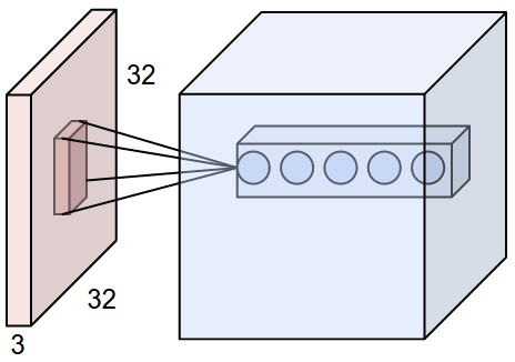
Example 1. For example, suppose that the input volume has size [32x32x3], (e.g. an RGB CIFAR-10 image). If the receptive field (or the filter size) is 5x5, then each neuron in the Conv Layer will have weights to a [5x5x3] region in the input volume, for a total of 5*5*3 = 75 weights (and +1 bias parameter). Notice that the extent of the connectivity along the depth axis must be 3, since this is the depth of the input volume.
Example 2. Suppose an input volume had size [16x16x20]. Then using an example receptive field size of 3x3, every neuron in the Conv Layer would now have a total of 3*3*20 = 180 connections to the input volume. Notice that, again, the connectivity is local in space (e.g. 3x3), but full along the input depth (20).

An example input volume in red (e.g. a 32x32x3 CIFAR-10 image), and an example volume of neurons in the first convolutional layer. Each neuron in the convolutional layer is connected only to a local region in the input volume spatially, but to the full depth (i.e. all color channels). Note, there are multiple neurons (5 in this example) along the depth, all looking at the same region in the input - see discussion of depth columns in text below.
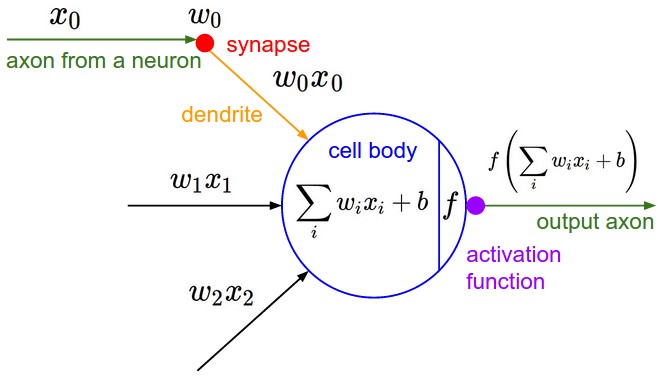
The neurons from the Neural Network chapter remain unchanged: They still compute a dot product of their weights with the input followed by a non-linearity, but their connectivity is now restricted to be local spatially.
Spatial arrangement
We have explained the connectivity of each neuron in the Conv Layer to the input volume, but we haven’t yet discussed how many neurons there are in the output volume or how they are arranged. Three hyperparameters control the size of the output volume: the depth, stride and zero-padding. We discuss these next:
- First, the depth of the output volume is a hyperparameter: it corresponds to the number of filters we would like to use, each learning to look for something different in the input. For example, if the first Convolutional Layer takes as input the raw image, then different neurons along the depth dimension may activate in presence of various oriented edged, or blobs of color. We will refer to a set of neurons that are all looking at the same region of the input as a depth column (some people also prefer the term fibre).
- Second, we must specify the stride with which we slide the filter. When the stride is 1 then we move the filters one pixel at a time. When the stride is 2 (or uncommonly 3 or more, though this is rare in practice) then the filters jump 2 pixels at a time as we slide them around. This will produce smaller output volumes spatially.
- As we will soon see, sometimes it will be convenient to pad the input volume with zeros around the border. The size of this zero-padding is a hyperparameter. The nice feature of zero padding is that it will allow us to control the spatial size of the output volumes (most commonly as we’ll see soon we will use it to exactly preserve the spatial size of the input volume so the input and output width and height are the same).
How to compute the number of neurons
We can compute the spatial size of the output volume as a function of the input volume size (W), the receptive field size of the Conv Layer neurons (F), the stride with which they are applied (S), and the amount of zero padding used (P) on the border. You can convince yourself that the correct formula for calculating how many neurons “fit” is given by (W − F + 2P) / S + 1. For example for a 7x7 input and a 3x3 filter with stride 1 and pad 0 we would get a 5x5 output. With stride 2 we would get a 3x3 output.
Use of zero-padding
In the example above on left, note that the input dimension was 5 and the output dimension was equal: also 5. This worked out so because our receptive fields were 3 and we used zero padding of 1. If there was no zero-padding used, then the output volume would have had spatial dimension of only 3, because that it is how many neurons would have “fit” across the original input. In general, setting zero padding to be P=(F−1)/2 when the stride is S=1 ensures that the input volume and output volume will have the same size spatially. It is very common to use zero-padding in this way and we will discuss the full reasons when we talk more about ConvNet architectures.
Constraints on strides. Note again that the spatial arrangement hyperparameters have mutual constraints. For example, when the input has size W=10, no zero-padding is used P=0, and the filter size is F=3, then it would be impossible to use stride S=2, since (W−F+2P)/S+1=(10−3+0)/2+1=4.5, i.e. not an integer, indicating that the neurons don’t “fit” neatly and symmetrically across the input. Therefore, this setting of the hyperparameters is considered to be invalid, and a ConvNet library could throw an exception or zero pad the rest to make it fit, or crop the input to make it fit, or something. As we will see in the ConvNet architectures section, sizing the ConvNets appropriately so that all the dimensions “work out” can be a real headache, which the use of zero-padding and some design guidelines will significantly alleviate.
Parameter Sharing
Parameter sharing scheme is used in Convolutional Layers to control the number of parameters. we can dramatically reduce the number of parameters by making one reasonable assumption: That if one feature is useful to compute at some spatial position (x,y), then it should also be useful to compute at a different position (x2,y2). In other words, denoting a single 2-dimensional slice of depth as a depth slice (e.g. a volume of size [55x55x96] has 96 depth slices, each of size [55x55]), we are going to constrain the neurons in each depth slice to use the same weights and bias.
Notice that if all neurons in a single depth slice are using the same weight vector, then the forward pass of the CONV layer can in each depth slice be computed as a convolution of the neuron’s weights with the input volume (Hence the name: Convolutional Layer). This is why it is common to refer to the sets of weights as a filter (or a kernel), that is convolved with the input.
Note that sometimes the parameter sharing assumption may not make sense. This is especially the case when the input images to a ConvNet have some specific centered structure, where we should expect, for example, that completely different features should be learned on one side of the image than another. One practical example is when the input are faces that have been centered in the image. You might expect that different eye-specific or hair-specific features could (and should) be learned in different spatial locations. In that case it is common to relax the parameter sharing scheme, and instead simply call the layer a Locally-Connected Layer.
